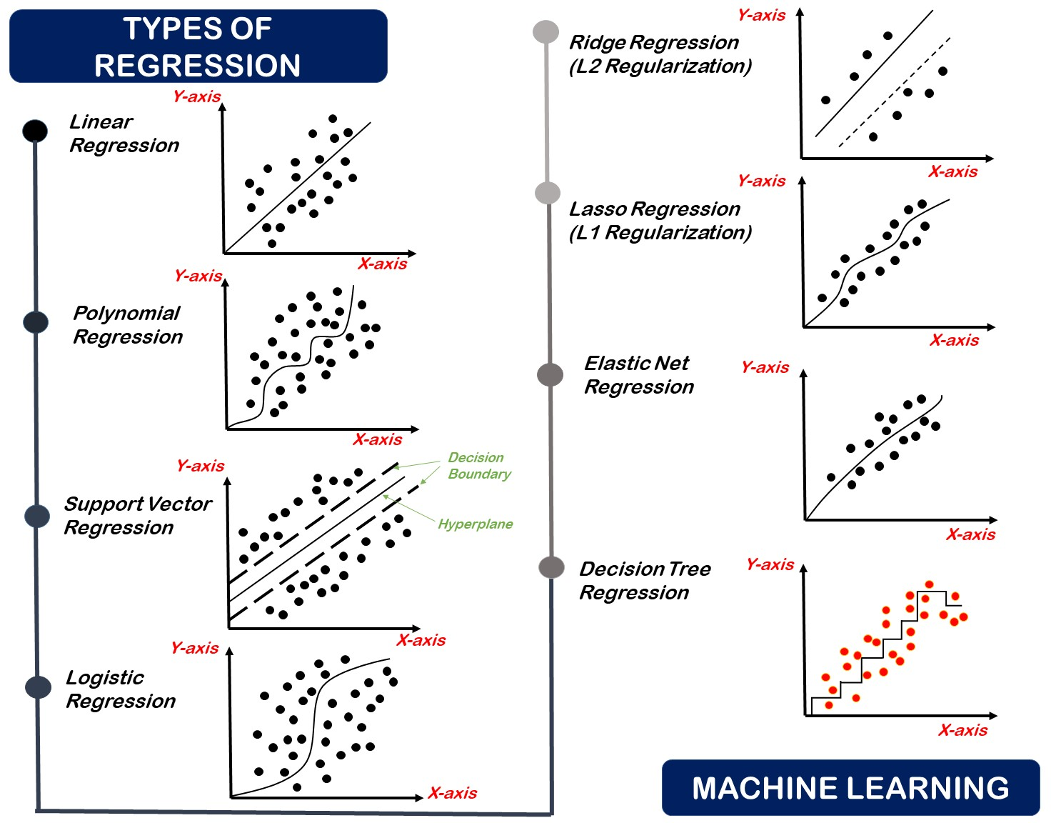
1. Regression using Linear line
The representation of linear regression is one of the most common and easiest algorithms of machine learning that read to the prediction modeling. It is a learning method used in supervised learning, and finds applications in statistics, economics or machine learning. It is a type of linear regression in which an equation that models with dependent variable also called (target) that relationship with one or more independent variables called (features) is fitted through the use of a line (known as the regression line) being drawn through the data points.
Linear regression aims at determining the best-fitting curve that would allow it to be used to predict output value (Y) on the basis of the input value(s) (X) and the equation is:
Y=aX+b Y = aX + bY = aX+b
In the equation defined as:
- Predicted value that is (Y)
- The input feature is (X)
- (a) is the gradient of the line (also known as coefficient)
- (b) is the intercept (the value of Y at X = 0)
The fact that linear regression is understandable and efficient is one of the reasons it is applied and used in many applications such as in forecasting, trend analysis and risk assessment.
Real-Life Example:
Predicting Blood Pressure Based on Age.
2. Polynomial Regression
Polynomial Regression is a type of linear regression, with independent variable relationships to the dependent variable being modeled as an nth order polynomial. It is applied where the relationship in the data is non-linear and cannot be well-described using a straight line (like in linear regression).
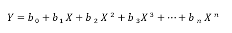
Polynomial regression fits a non-linear curve, or series of linear functions, and the form of the curve is given by:
In a polynomial regression equation, Y represents the predicted output, X is the input feature, b₀, b₁, …, bₙ are the coefficients, and n indicates the number of terms in the polynomial.
Polynomial regression enables the model to fit more complex data trends than linear regression, but selecting an overly large degree might result in overfitting the data, which is when models do very well on the training dataset however fail to simplify on the novel data.
Real-Life Example:
Modeling vehicle speed vs. fuel efficiency (MPG), where the curve best fits the pattern.
3. Support Vector Regression (SVR)
The Support Vector Machine (SVM) is an algorithms and Support Vector Regression (SVR) is part of this algorithm that applied to regression. SVR, unlike traditional regression models which attempt to reduce the error between the predictions and the actuals attempts to fit the line(in lower-dimensional data) or hyperplane(in higher-dimensional data) that best fits within a margin of tolerance (epsilon) about the actual data points.
The main principle of SVR is to make the model predict values, which are not too different than the real outputs, but still give some space (delta determined by epsilon) to errors. Simultaneously, it also attempts to maximize the margin of the hyperplane which makes it more robust and generalizable.
SVR is especially powerful for:
- Handling non-linear relationships, using kernel functions like RBF (Radial Basis Function)
- Working well with high-dimensional data
- Providing better control over model complexity and error tolerance
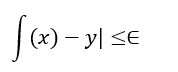
Mathematically, the goal of Support Vector Regression is to put a function f(x) as follows:
while keeping the model as flat as possible.
Real-Life Example:
Estimate today’s air quality based on weather readings.
4. Regression using Logistic
A classification method in regression using logistic is both a classification problem and a classification algorithm of the type called supervised learning. It is referred to as logistic because it is the kind of prediction that is applied to find out the chance that a numerical value outcome takes place e.g., yes/no, spam/not spam, disease/no disease etc.
As opposed to linear regression that makes predictions on the continuous values of bands, logistic regressions make predictions on the likelihood of the input falling in one class. It uses the logistic (sigmoid) function, which maps any real number to the range [ 0, 1 ] ; hence it is especially well-suited to binary classification.
The well know Sigmoid function is.:
In which representation of z is the input feature in a linear combination. When the probability of the output is larger than 0.5, the model output is class 1, otherwise class 0.
There are many Logistic Regression applications are due to the fact that:
- Easy and resourceful
- Interpretable
- Linearly separable data is effective
It may also be extended to multiclass settings in through such methods as One-vs-Rest (OvR).
Real-Life Example:
Classification of emails (Spam or not spam).
Or
Predicting Heart Disease
5. Decision Tree Regression
One of the supervised learning methods that is employed in making predictions on continuous values regressions task is Decision Tree Regression method. It splits the dataset in smaller parts using decision rules, and at each node it will output a simple number instead of class label.
The algorithm forms a hierarchy-like sequence of data:
- The internal vertex is a feature quash decision
- Each branch is representing decision outcome
- All the leaf nodes represent contingent values
Model splits data to split data of such a way that it decreases the mean squared error (MSE) or other regression loss functions at each node.
The popularity of Decision Tree Regression is associated with the fact that it:
- Is simple to read and picture out
- Ability to capture non-linear relationship
- It does not necessarily need much data preprocessing
But when a tree is excessively deep it can overfit the training data, making the prediction of the tree to new examples inconsequential, this leads to the common practice of pruning the tree or using depth limits.
Real-Life Example:
Predicting Time to Complete a Task Based on Skill Level.
6. Elastic Net Regression in Machine Learning
Regularized regression method that encompasses the L1 (Lasso) and L2 (Ridge) penalization in the same model is referred to as Elastic Net Regression. One may rely on it where it is necessary to improve accuracy of predictions and interpretability of linear models where either the number of features is high, or featured variables represent sets of very correlated variables.
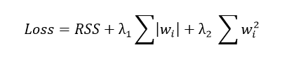
The Elastic Net cost function is:
Where:
- RSS is the remaining quantity of squares (the main error term)